Where does probably fit in?

Introduction

An obvious question regarding probably might be: where does this fit in with the rest of the tidymodels ecosystem? Like the other pieces of the ecosystem, probably is designed to be modular, but plays well with other tidymodels packages.

Regarding placement in the modeling workflow, probably best fits in as a post processing step after the model has been fit, but before the model performance has been calculated.

Example

As an example, we’ll use parsnip to fit a logistic regression on some Lending Club https://www.lendingclub.com/ loan data, and then use probably to investigate what happens to performance when you vary the threshold of what a “good” loan is.

library(parsnip)
library(probably)
library(dplyr)
library(rsample)
library(modeldata)
data("lending_club")

# I think it makes more sense to have "good" as the first level
# By default it comes as the second level
lending_club <- lending_club %>%
  mutate(Class = relevel(Class, "good"))

# There are a number of columns in this data set, but we will only use a few
# for this example
lending_club <- select(lending_club, Class, annual_inc, verification_status, sub_grade)

lending_club
#> # A tibble: 9,857 × 4
#>    Class annual_inc verification_status sub_grade
#>    <fct>      <dbl> <fct>               <fct>    
#>  1 good       35000 Not_Verified        C4       
#>  2 good       72000 Verified            C1       
#>  3 good       72000 Source_Verified     D1       
#>  4 good      101000 Verified            C3       
#>  5 good       50100 Source_Verified     A4       
#>  6 good       32000 Source_Verified     B5       
#>  7 good       65000 Not_Verified        A1       
#>  8 good      188000 Not_Verified        B2       
#>  9 good       89000 Source_Verified     B3       
#> 10 good       48000 Not_Verified        C2       
#> # ℹ 9,847 more rows

Let’s split this into 75% training and 25% testing for something to predict on.

# 75% train, 25% test
set.seed(123)

split <- initial_split(lending_club, prop = 0.75)

lending_train <- training(split)
lending_test <- testing(split)

Before we do anything, let’s look at the counts of what we are going to be predicting, the Class of the loan.

count(lending_train, Class)
#> # A tibble: 2 × 2
#>   Class     n
#>   <fct> <int>
#> 1 good   7008
#> 2 bad     384

Clearly there is a large imbalance here with the number of good and bad loans. This is probably a good thing for the bank, but poses an interesting issue for us because we might want to ensure we are sensitive to the bad loans and are not overwhelmed by the number of good ones. One thing that we might do is downsample the number of good loans so that the total number of them is more in line with the number of bad loans. We could do this before fitting the model using themis::step_downsample(), but for now, let’s continue with the data unchanged.

We’ll use parsnip’s logistic_reg() to create a model specification for logistic regression, set the engine to be glm and then actually fit the model using our data and the model formula.

logi_reg <- logistic_reg()
logi_reg_glm <- logi_reg %>% set_engine("glm")

# A small model specification that defines the type of model you are
# using and the engine
logi_reg_glm
#> Logistic Regression Model Specification (classification)
#> 
#> Computational engine: glm

# Fit the model
logi_reg_fit <- fit(
  logi_reg_glm,
  formula = Class ~ annual_inc + verification_status + sub_grade,
  data = lending_train
)

logi_reg_fit
#> parsnip model object
#> 
#> 
#> Call:  stats::glm(formula = Class ~ annual_inc + verification_status + 
#>     sub_grade, family = stats::binomial, data = data)
#> 
#> Coefficients:
#>                        (Intercept)                          annual_inc  
#>                         -5.670e+00                           1.915e-06  
#> verification_statusSource_Verified         verification_statusVerified  
#>                          4.324e-02                           3.364e-01  
#>                        sub_gradeA2                         sub_gradeA3  
#>                          9.508e-02                           1.149e+00  
#>                        sub_gradeA4                         sub_gradeA5  
#>                         -5.591e-02                           1.510e+00  
#>                        sub_gradeB1                         sub_gradeB2  
#>                          1.637e+00                           1.177e+00  
#>                        sub_gradeB3                         sub_gradeB4  
#>                          1.467e+00                           1.975e+00  
#>                        sub_gradeB5                         sub_gradeC1  
#>                          2.125e+00                           2.234e+00  
#>                        sub_gradeC2                         sub_gradeC3  
#>                          2.176e+00                           2.380e+00  
#>                        sub_gradeC4                         sub_gradeC5  
#>                          2.724e+00                           3.084e+00  
#>                        sub_gradeD1                         sub_gradeD2  
#>                          3.105e+00                           2.816e+00  
#>                        sub_gradeD3                         sub_gradeD4  
#>                          3.165e+00                           3.125e+00  
#>                        sub_gradeD5                         sub_gradeE1  
#>                          3.507e+00                           3.621e+00  
#>                        sub_gradeE2                         sub_gradeE3  
#>                          3.272e+00                           3.542e+00  
#>                        sub_gradeE4                         sub_gradeE5  
#>                          3.428e+00                           3.468e+00  
#>                        sub_gradeF1                         sub_gradeF2  
#>                          3.717e+00                           4.096e+00  
#>                        sub_gradeF3                         sub_gradeF4  
#>                          3.681e+00                           3.662e+00  
#>                        sub_gradeF5                         sub_gradeG1  
#>                          3.586e+00                           4.168e+00  
#>                        sub_gradeG2                         sub_gradeG3  
#>                          4.162e+00                           4.422e+00  
#>                        sub_gradeG4                         sub_gradeG5  
#>                          5.102e+00                          -8.226e+00  
#> 
#> Degrees of Freedom: 7391 Total (i.e. Null);  7354 Residual
#> Null Deviance:       3019 
#> Residual Deviance: 2716  AIC: 2792

The output of the parsnip fit() call is a parsnip model_fit object, but the underlying print method for the glm fit is used.

Now let’s predict on our testing set, and use type = "prob" to get class probabilities back rather than hard predictions. We will use these with probably to investigate performance.

predictions <- logi_reg_fit %>%
  predict(new_data = lending_test, type = "prob")

head(predictions, n = 2)
#> # A tibble: 2 × 2
#>   .pred_good .pred_bad
#>        <dbl>     <dbl>
#> 1      0.969    0.0311
#> 2      0.965    0.0353

lending_test_pred <- bind_cols(predictions, lending_test)

lending_test_pred
#> # A tibble: 2,465 × 6
#>    .pred_good .pred_bad Class annual_inc verification_status sub_grade
#>         <dbl>     <dbl> <fct>      <dbl> <fct>               <fct>    
#>  1      0.969   0.0311  good       32000 Source_Verified     B5       
#>  2      0.965   0.0353  good       73400 Source_Verified     C2       
#>  3      0.960   0.0405  good      175000 Source_Verified     B5       
#>  4      0.972   0.0276  good       70000 Not_Verified        B4       
#>  5      0.874   0.126   good       36000 Source_Verified     E1       
#>  6      0.944   0.0560  good       40000 Source_Verified     C4       
#>  7      0.996   0.00385 good       60000 Not_Verified        A1       
#>  8      0.951   0.0486  good       65000 Verified            C1       
#>  9      0.963   0.0370  good       52000 Verified            B4       
#> 10      0.983   0.0173  good       61000 Verified            B2       
#> # ℹ 2,455 more rows

With our class probabilities in hand, we can use make_two_class_pred() to convert these probabilities into hard predictions using a threshold. A threshold of 0.5 just says that if the predicted probability is above 0.5, then classify this prediction as a “good” loan, otherwise, bad.

hard_pred_0.5 <- lending_test_pred %>%
  mutate(
    .pred = make_two_class_pred(
      estimate = .pred_good,
      levels = levels(Class),
      threshold = .5
    )
  ) %>%
  select(Class, contains(".pred"))

hard_pred_0.5 %>%
  count(.truth = Class, .pred)
#> # A tibble: 2 × 3
#>   .truth      .pred     n
#>   <fct>  <clss_prd> <int>
#> 1 good         good  2332
#> 2 bad          good   133

Hmm, with a 0.5 threshold, almost all of the loans were predicted as “good”. Perhaps this has something to do with the large class imbalance. On the other hand, the bank might want to be more stringent with what is classified as a “good” loan, and might require a probability of 0.75 as the threshold.

hard_pred_0.75 <- lending_test_pred %>%
  mutate(
    .pred = make_two_class_pred(
      estimate = .pred_good,
      levels = levels(Class),
      threshold = .75
    )
  ) %>%
  select(Class, contains(".pred"))

hard_pred_0.75 %>%
  count(.truth = Class, .pred)
#> # A tibble: 4 × 3
#>   .truth      .pred     n
#>   <fct>  <clss_prd> <int>
#> 1 good         good  2320
#> 2 good          bad    12
#> 3 bad          good   129
#> 4 bad           bad     4

In this case, 4 of the bad loans were correctly classified as bad, but more of the good loans were also misclassified as bad now. There is a tradeoff here, which can be somewhat captured by the metrics sensitivity and specificity. Both metrics have a max value of 1.

sensitivity - The proportion of predicted “good” loans out of all “good” loans
specificity - The proportion of predicted “bad” loans out of all “bad” loans

library(yardstick)

sens(hard_pred_0.5, Class, .pred)
#> # A tibble: 1 × 3
#>   .metric .estimator .estimate
#>   <chr>   <chr>          <dbl>
#> 1 sens    binary             1
spec(hard_pred_0.5, Class, .pred)
#> # A tibble: 1 × 3
#>   .metric .estimator .estimate
#>   <chr>   <chr>          <dbl>
#> 1 spec    binary             0

sens(hard_pred_0.75, Class, .pred)
#> # A tibble: 1 × 3
#>   .metric .estimator .estimate
#>   <chr>   <chr>          <dbl>
#> 1 sens    binary         0.995
spec(hard_pred_0.75, Class, .pred)
#> # A tibble: 1 × 3
#>   .metric .estimator .estimate
#>   <chr>   <chr>          <dbl>
#> 1 spec    binary        0.0301

In this example, as we increased specificity (by capturing those 4 bad loans with a higher threshold), we lowered sensitivity (by incorrectly reclassifying some of the good loans as bad). It would be nice to have some combination of these metrics to represent this tradeoff. Luckily, j_index is exactly that.

\[ j\_index = sens + spec - 1 \]

j_index has a maximum value of 1 when there are no false positives and no false negatives. It can be used as justification of whether or not an increase in the threshold value is worth it. If increasing the threshold results in more of an increase in the specificity than a decrease in the sensitivity, we can see that with j_index.

j_index(hard_pred_0.5, Class, .pred)
#> # A tibble: 1 × 3
#>   .metric .estimator .estimate
#>   <chr>   <chr>          <dbl>
#> 1 j_index binary             0
j_index(hard_pred_0.75, Class, .pred)
#> # A tibble: 1 × 3
#>   .metric .estimator .estimate
#>   <chr>   <chr>          <dbl>
#> 1 j_index binary        0.0249

Now, this is not the only way to optimize things. If you care about low false positives, you might be more interested in keeping sensitivity high, and this wouldn’t be the best way to tackle this problem. But for now, let’s see how we can use probably to optimize the j_index.

threshold_perf() will recalculate a number of metrics across varying thresholds. One of these is j_index.

threshold_data <- lending_test_pred %>%
  threshold_perf(Class, .pred_good, thresholds = seq(0.5, 1, by = 0.0025))

threshold_data %>%
  filter(.threshold %in% c(0.5, 0.6, 0.7))
#> # A tibble: 9 × 4
#>   .threshold .metric     .estimator .estimate
#>        <dbl> <chr>       <chr>          <dbl>
#> 1        0.5 sensitivity binary        1     
#> 2        0.6 sensitivity binary        0.999 
#> 3        0.7 sensitivity binary        0.998 
#> 4        0.5 specificity binary        0     
#> 5        0.6 specificity binary        0.0226
#> 6        0.7 specificity binary        0.0226
#> 7        0.5 j_index     binary        0     
#> 8        0.6 j_index     binary        0.0217
#> 9        0.7 j_index     binary        0.0208

With ggplot2, we can easily visualize this varying performance to find our optimal threshold for maximizing j_index.

library(ggplot2)

threshold_data <- threshold_data %>%
  filter(.metric != "distance") %>%
  mutate(group = case_when(
    .metric == "sens" | .metric == "spec" ~ "1",
    TRUE ~ "2"
  ))

max_j_index_threshold <- threshold_data %>%
  filter(.metric == "j_index") %>%
  filter(.estimate == max(.estimate)) %>%
  pull(.threshold)

ggplot(threshold_data, aes(x = .threshold, y = .estimate, color = .metric, alpha = group)) +
  geom_line() +
  theme_minimal() +
  scale_color_viridis_d(end = 0.9) +
  scale_alpha_manual(values = c(.4, 1), guide = "none") +
  geom_vline(xintercept = max_j_index_threshold, alpha = .6, color = "grey30") +
  labs(
    x = "'Good' Threshold\n(above this value is considered 'good')",
    y = "Metric Estimate",
    title = "Balancing performance by varying the threshold",
    subtitle = "Sensitivity or specificity alone might not be enough!\nVertical line = Max J-Index"
  )

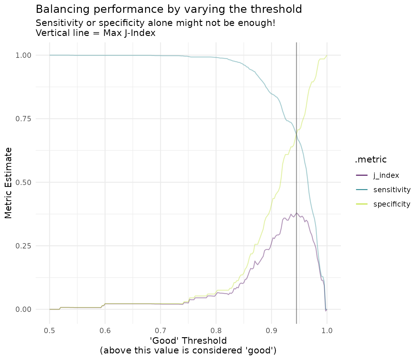
It’s clear from this visual that the optimal threshold is very high, exactly 0.945. This is pretty high, so again, this optimization method won’t be useful for all cases. To wrap up, here are all of the test set metrics for that threshold value.

threshold_data %>%
  filter(.threshold == max_j_index_threshold)
#> # A tibble: 3 × 5
#>   .threshold .metric     .estimator .estimate group
#>        <dbl> <chr>       <chr>          <dbl> <chr>
#> 1      0.945 sensitivity binary         0.687 2    
#> 2      0.945 specificity binary         0.692 2    
#> 3      0.945 j_index     binary         0.379 2

Davis Vaughan

2024-02-23

Introduction

Example